
We used to have fftw…
Published:
This article offers a pragmatic overview of the Fast Fourier Transform (FFT) for developers of scientific software.
1. Basics
The Discrete Fourier Transform (DFT) of a one-dimensional vector \(x \in \mathbb{C}^N\) is another vector \(X \in \mathbb{C}^N\) defined by
\[ X_k = \sum_{j=0}^{N-1} x_j \, \omega_N^{jk}, \quad k = 0, 1, \dots, N-1, \]
where
\[ \omega_N \triangleq e^{-2\pi i / N}. \]
Whereas the direct implementation of the DFT requires \(O(N^2)\) operations, it can be decomposed into smaller DFTs when \(N\) is a composite number, leading to a faster implementation.
For example, when \(N\) is even, the DFT formula can be rewritten as
\[ X_k = \sum_{j’=0}^{\frac{N}{2}-1} x_{2j’} \, \omega_{\frac{N}{2}}^{j’k} + \omega_N^{k} \sum_{j’=0}^{\frac{N}{2}-1} x_{2j’+1} \, \omega_{\frac{N}{2}}^{j’k}. \]
This means that, if you already have the DFTs of the two halves \(\{x_{2j'}\}_{j' = 0,1,\dots,\frac{N}{2}-1}\) and \(\{x_{2j'+1}\}_{j' = 0,1,\dots,\frac{N}{2}-1},\) then you can combine them with the cost of \(O(N)\) operations to obtain the DFT of the whole sequence. If \(N\) is a power of 2, you can recursively apply this decomposition, and the computational cost of DFT \(T(N)\) satisfies \(T(N) = 2T(\frac{N}{2}) + O(N)\) whose solution is \(T(N) = O(N \log N)\).
This decomposition is known as the Cooley–Tukey algorithm 1. Even for prime \(N\), the DFT of \(x \in \mathbb{C}^N\) can be reduced to DFTs with some factorizable length \(N'\) by Rader’s algorithm 2 or Bluestein’s algorithm 3. Common FFT libraries combine these approaches and dispatch optimal FFT code depending on the shape of input data. For example, the PocketFFT library — used in both numpy.fft and scipy.fft — implements the Cooley–Tukey algorithm for composite lengths with small factors (e.g., \(r = 2, 3, 5, 7, 11\)), and switches to Bluestein’s algorithm for large prime factors.
2. High Performance FFT
The optimal FFT algorithm depends not only on the shape of the data, but also on the machine that executes it. This idea forms the foundation of the well-known FFTW library, which achieves performance comparable to vendor-tuned implementations such as Intel’s MKL FFT, by adaptively searching for the best algorithm for any given computing environment. Although this article cannot cover all of FFTW’s technical aspects, this chapter aims to provide a concise explanation of how FFT performance is tied to hardware characteristics.
Hierarchical Memory
When analyzing the performance of computational algorithms, it is often found that a significant portion of execution time is spent transferring data between the processor and the main memory, rather than performing arithmetic itself. A fundamental approach to this problem is the hierarchical memory system. If a program repeatedly accesses the same data, that data should be kept close to the processor — in the cache, a small but extremely fast memory. This hierarchy, typically consisting of several levels (L1, L2, L3), is designed to bridge the enormous speed gap between the CPU and the main memory.
Although caching remains an essential technique for programmers today, its relative importance has changed since the era of FFTW. The reasons are:
- The performance of hierarchical memory has drastically improved, both in cache capacity and memory bandwidth.
- Parallel computing (such as GPUs) has become the dominant factor in high-performance computing.
The optimization strategy in FFTW can be summarized, in a nutshell, as an effort to maximize cache efficiency. While today’s computing environments differ greatly from the architectures for which FFTW was originally optimized, there is still much to learn from its underlying philosophy.
Depth-First vs. Breadth-First
As described in the previous section, the Cooley–Tukey algorithm decomposes a DFT into smaller DFTs. For the radix-2 case, this decomposition can be represented as a binary tree, where each node corresponds to a subproblem.
There are two natural ways to traverse this tree:
- Breadth-first approach: compute all DFTs at the same level before proceeding to the next.
- Depth-first approach: recursively compute a full branch of the tree before moving to another.
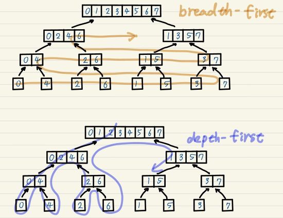
The key observation presented in the FFTW paper 4 is that the depth-first traversal is more cache-efficient, since it tends to work on a small subset of the entire data. The authors also note that the optimal factorization of \(N\) depends on hardware details such as cache capacity and latency, and thus should be determined through auto-tuning.
FFTW today
From an economic viewpoint, the development of auto-tuning libraries such as FFTW or SPIRAL5 was partly motivated by the diversity of CPU architectures — different vendors such as Intel and AMD required different low-level optimizations. However, FFT is a task that benefits enormously from GPU acceleration, and the GPU ecosystem today is overwhelmingly dominated by NVIDIA. In such a landscape, NVIDIA’s vendor-optimized cuFFT library is often sufficient for most applications.
That said, when performing FFTs of very large problem sizes in CPU-only environments, FFTW still remains one of the best choices today.
3. FFT in Practice
This chapter illustrates how to work with FFTs in Python, with a focus on switching between different backends.
FFT Libraries in Python
SciPy
scipy.fftuses PocketFFT as its engine. AlthoughNumPyrelies on the same backend, a practical difference is thatnumpy.fftalways returns double-precision arrays, even when the input is single precision. Therefore, those who want to control the dtype for performance (like me) should usescipy.fft.pyFFTW
pyfftwis a Python wrapper around FFTW and provides convenient interfaces such aspyfftw.interfaces.numpy_fftandpyfftw.interfaces.scipy_fftpack. In this blog, however, a sample code that directly interacts with thepyfftw.FFTWobject — which holds the optimal FFT algorithm determined by auto-tuning (the plan in FFTW’s terminology) — will be presented.CuPy
CuPyis a NumPy/SciPy-compatible array library developed by Preferred Networks as the backend ofChainer, a pioneering define-by-run deep learning framework. Although Chainer was eventually overtaken by PyTorch,CuPyremains an invaluable tool in the scientific computing community.cupy.fftuses cuFFT as its backend, and while cuFFT itself features auto-tuning mechanisms similar to FFTW, CuPy (≥ v8) implicitly caches FFT plans by default — meaning you can benefit from tuning without ever thinking about it.
Abstracting FFT Backends
Thanks to the NumPy-compatible API of CuPy, switching between CPU and GPU array backends is not difficult. A minimal example is available in fft_comparison/array_backend.py. The essence of this code is to maintain the array backend as a global variable. In the example below, the global _backend_module is initialized as numpy:
    import numpy as _np

    _backend_name = "numpy"
    _backend_module = _np
By defining set_array_backend() and get_array_backend() to interact with _backend_module, you can switch between numpy and cupy.
To interact with pyfftw, scipy.fft, and cupy.fft from a unified interface, a minimum object-oriented abstraction for FFT backends is shown in fft_comparison/fft_backend.py. In this sample code, only two-dimensional fft and ifft are implemented:
    class FFTBackend:
        """Abstract FFT backend interface."""

        def fft2(self, x: Any) -> Any:
            raise NotImplementedError

        def ifft2(self, x: Any) -> Any:
            raise NotImplementedError

        def __repr__(self) -> str:
            return self.__class__.__name__
Subclassing FFTBackend for scipy and cupy backends is straightforward. For pyfftw, an additional _get_plan() method is introduced to initialize and cache plans:
    def _get_plan(self, shape: Tuple[int, ...], dtype: Any, direction: str):
        key = (shape, dtype, direction)
        if key not in self._plans:
            a = self.pyfftw.empty_aligned(shape, dtype=dtype)
            b = self.pyfftw.empty_aligned(shape, dtype=dtype)
            fftw_dir = "FFTW_FORWARD" if direction == "fft" else "FFTW_BACKWARD"
            plan = self.pyfftw.FFTW(
                a,
                b,
                axes=(-2, -1),
                direction=fftw_dir,
                threads=self.threads,
                flags=(self.planner_effort,),
            )
            self._plans[key] = (plan, a, b)
        return self._plans[key]
This method is called within fft2 and ifft2, and a new plan is constructed only when a new combination of (shape, dtype, direction) is encountered.
4. FFT Dominates?
A conventional argument in image-processing performance analysis is the so-called O(N log N) argument. The reason for this is that many fundamental image-processing workloads consist of FFTs with \(O(N \log N)\) complexity and other accompanying \(O(N)\) operations. So the argument is that, for sufficiently large \(N\), the FFT should dominate the overall computational cost. However, what matters in science is a quantitative verification. So, let’s measure how much time FFTs actually consume using the unified code base presented in the previous chapter.
Benchmark Design
Each iteration consisted of three stages:
- FFT forward + inverse \(b = \mathrm{FFT}(a), \quad a_\text{recon} = \mathrm{IFFT}(b)\)
- Element-wise arithmetic \(\text{diff} = |a - a_\text{recon}|^2\)
- Reduction \(s = \sum \text{diff}\)
The total runtime and the relative share of each stage were recorded. For CPU runs, profiling was performed using Python’s cProfile; for GPU runs, CUDA event–based timing measured device-side kernel durations.
Summary of FFT Share
The following table summarizes the fraction of total runtime spent in the FFT stage (%) for each backend and image size. Detailed profiling results, including element-wise and reduction costs, are available in the repository: fft_comparison/README.md.
| FFT Backend | 256×256 | 512×512 | 1024×1024 |
|---|---|---|---|
| SciPy (PocketFFT) | 86 % | 72 % | 76 % |
| pyFFTW (1 thread) | 88 % | 67 % | 68 % |
| pyFFTW (4 threads) | 89 % | 60 % | 56 % |
| CuPy (cuFFT) | 39 % | 56 % | 89 % |
It is worth noting that the non-FFT parts in this benchmark are extremely simple, and yet their contribution is not negligible under most conditions. This implies that in more realistic workloads, where preprocessing and postprocessing are usually more complex, the relative share of FFT would likely be even smaller. Therefore, before optimizing FFT itself, developers should verify whether FFT is truly the performance bottleneck. (As a practical note, in GPU computing, such post-processing following FFT can often be further optimized through kernel fusion.)
References
An Algorithm for the Machine Calculation of Complex Fourier Series.
Mathematics of Computation, 19(90), 297–301.
https://doi.org/10.2307/2003354
Discrete Fourier transforms when the number of data samples is prime.
Proceedings of the IEEE, 56(6), 1107–1108.
https://doi.org/10.1109/PROC.1968.6477
A linear filtering approach to the computation of discrete Fourier transform.
IEEE Transactions on Audio and Electroacoustics, 18(4), 451–455.
https://doi.org/10.1109/TAU.1970.1162132
The Design and Implementation of FFTW3. Proceedings of the IEEE, 93(2), 216-231. https://doi.org/10.1109/JPROC.2004.840301
SPIRAL: Extreme Performance Portability. Proceedings of the IEEE, 106(11), 1935-1968 https://doi.org/10.1109/JPROC.2018.2873289