Implementing Message Passing Algorithms

Probabilistic Programming Languages (PPLs) automate inference on probabilistic models defined by its users. Implementing such a software framework sounds pretty daunting, because no algorithm is universally applicable or scalable to arbitrary inference tasks. General purpose PPLs, such as Turing.jl and Numpyro, support multiple methods including MCMC and variational inference, to cover a wide range of problems.

This article, however, focuses on the message passing libraries, such as Infer.NET and ForneyLab.jl. Although the space of problems that these libraries can handle is much smaller than PPLs, they support scalable inference for high-dimensional models commonly found in time-series analysis and computational imaging.

1. Basics

This section overviews the sum-product algorithm and its variants. To establish the notation, we consider a joint distribution of a set of variables \(\mathcal{V} = \{ X_1, X_2, \cdots, X_N \}\). Computing the marginal distribution of \(X_i (i = 1,2,\cdots, N)\) by the direct integration over \(\mathcal{V} - \{X_i\}\) would come with an exponentially large cost. To avoid this, we assume that the joint distribution is factorized as

where \(X_{\mathcal{V}} = (X_1, X_2, \cdots, X_N )\), \(\mathcal{F}\) is a finite set of factors, and \(X_f\) denotes the collection of variables that constitute the arguments of the factor \(f \in \mathcal{F}\). \(Z\) is the normalizing constant, and we want an inference algorithm that can be implemented without the knowledge about \(Z\).

Such a structure can be expressed as a bipartite graph, where each factor node is connected to the variable nodes that appear in its argument. This graph is known as the factor graph, and specified by the set of variables \(\mathcal{V}\), the set of factors \(\mathcal{F}\), and the set of edges \(\mathcal{E} \subset \mathcal{V} \times \mathcal{F}\):

A factor graph representing \(p(X_1, X_2, X_3) \propto f_1(X_1) f_2(X_1, X_2, X_3) f_3(X_2) f_4(X_3)\) is illustrated below.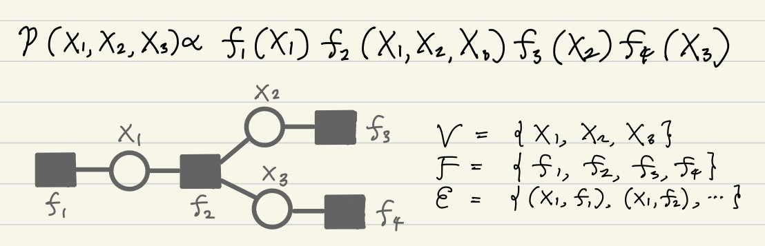

Assuming that a factor graph \(\mathcal{G}\) has no loops, the marginal distribution of \(X_i\) is expressed as a product of contributions from smaller subtrees. To see this, suppose that \(X_i\) node is associated with three factors \(f_1, f_2\), and \(f_3\). We denote the subgraph consisting of nodes that can be reached from \(X_i\) through \(f_j (j = 1,2,3)\) by \(\mathcal{G}_j\).

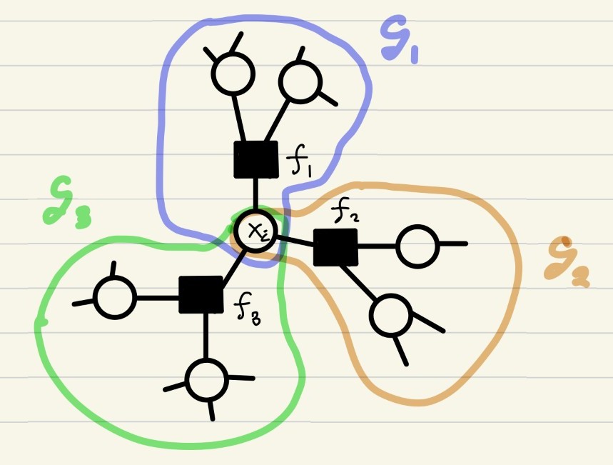
Then, it follows that \(p(X_i)\) is simply the product of marginal distributions w.r.t. subtrees \(\mathcal{G}_1, \mathcal{G}_2, \mathcal{G}_3\):

where \(\mathcal{G}_j = (\mathcal{V}_j, \mathcal{F}_j, \mathcal{E}_j) (j = 1,2,3)\). The distribution \(M_{f_j \rightarrow X_i}\) is referred to as the message sent from \(f_j\) to \(X_i\). This sounds like a nice divide-and-conquer approach.

Next, we ask whether the computation of \(M_{f_j \rightarrow X_i} (x_j)\) can be decomposed further. Suppose that the factor nodes \(f_j\) is associated with \(X_i\) and other variable nodes \(X_a, X_b, X_c\), and denote by \(\mathcal{G}_a, \mathcal{G}_b, \mathcal{G}_c\) the subtree of \(\mathcal{G}_j\) that can be reached from \(X_a, X_b, X_c\) without traversing the factor \(f_j\).

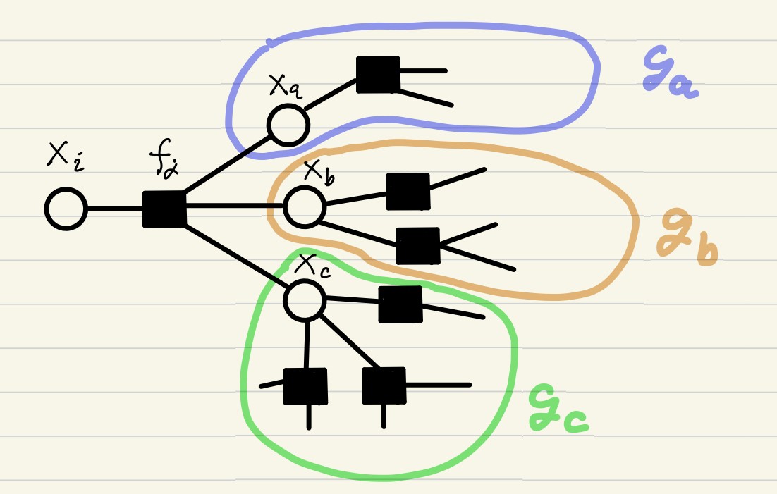
Then the message is computed as

where each variable-to-factor message is defined by

with \(\mathcal{G}_s = (\mathcal{V}_s, \mathcal{F}_s, \mathcal{E}_s) (s = a,b,c)\). Obviously, the computation of \(M_{X_s \rightarrow f_j} (x_s)\) can be further decomposed in the same manner.

To summarize, the computation of \(p(x_i)\) reduces to a sequence of low-dimensional integrations and products over the local neighborhoods in the factor graph. The messages \(M_{X \rightarrow f}\) and \(M_{f \rightarrow X}\), obtained as byproducts of computing \(p(x_i)\), can be used for computing the marginals of other variable nodes. Thus, since we are smart programmers, we should record the values of those messages. (This is what dynamic programming is all about.) In a formal expression, the sum-product algorithm recursively applies these update rules for all \((X, f) \in \mathcal{E}\) until convergence.

where \(\mathcal{F}_X\) and \(\mathcal{V}_f\) denote factor nodes associated with \(X \in \mathcal{V}\) and variable nodes associated with \(f \in \mathcal{F}\). When it converges, the marginal of \(X\) is estimated as \(p(x) \propto \prod_{f \in \mathcal{F}_X} M_{f \rightarrow X}\), whereas the joint distribution of \(\mathcal{V}_f\) is given by \(p(X_f) \propto f(X_f) \prod_{X \in \mathcal{V}_f} M_{X \rightarrow f} (x)\)

There are many inference algorithms in the spirit of the sum-product framework. For continuous variables, exact messages are typically intractable because general pdfs cannot be stored or processed on a computer. Expectation Propagation (EP)¹ approximates messages by members of an exponential family, whereas particle-filter–type algorithms can be viewed as representing messages as weighted sums of Dirac masses². When the sum step in the sum–product update is analytically intractable, one may combine it with a naive-variational-Bayes–like approximation to compute the message, yielding Variational Message Passing (VMP)³. For in-depth review on these topics, please refer to Pattern Recognition and Machine Learning⁴, Information, Physics, and Computation⁵, and Graphical Models, Exponential Families, and Variational Inference⁶.

2. Software abstraction

The sum–product algorithm has a structure that lends itself naturally to object-oriented programming (OOP): one may define a variable class and a factor class, where the former performs the product update and the latter performs the sum update. This section examines how such an abstraction can be realized in practice, with examples from ForneyLab.jl⁷ and my ongoing project gPIE.

The base classes

Let us consider the minimal design of the variable class and the factor class. What sort of data and operations should these objects have? A variable object should, at the very least, keep references to the factor nodes it is connected to. In Python, such a minimal class may look like the following:

    class Variable:
        def __init__(self, vid):
            self.id: int = vid                # integer identifier
            self.associated_factors: List[Factor] = [] # list of Factor objects

Likewise, the factor class may look like this:

    class Factor:
        def __init__(self, fid):
            self.id: int = fid                # integer identifier
            self.associated_variables: List[Variable] = [] # list of Variable objects

For simplicity, let us restrict all variable nodes to take values in \(\mathbf{R}\), and assume that all messages are represented by Gaussian distributions (this corresponds to the Gaussian case of Expectation Propagation). It would be convenient if we could treat a Gaussian distribution as an object:

    class Gaussian:
        def __init__(self, mean, variance):
            if variance < 0:
                raise RuntimeError("Negative variance!")
            self.mean: float = mean
            self.variance: float = variance

In sum-product algorithm, we frequently compute the product and the division of pdfs, thus it would be nice if it is expressed as a binary operation between Gaussian objects.

    class Gaussian:
        ....
        def __mul__(self: Gaussian, other: Gaussian):
            """
            Usage: Gaussian_prod = Gaussian_l * Gaussian_r
            """
            product_variance = 1/(1/self.variance + 1/other.variance)
            product_mean = (self.mean/self.variance + other.mean/other.variance) * product_variance
            return Gaussian(mean = product_mean, variance = product_variance)

        def __truediv__(self: Gaussian, other: Gaussian):
            """
            Usage: Gaussian_div = Gaussian_l / Gaussian_r
            """
            division_variance = 1/(1/self.variance - 1/other.variance)
            division_mean = (self.mean/self.variance - other.mean/other.variance) * division_variance
            return Gaussian(mean = division_mean, variance = division_variance)

A clear problem with this code is that, in __truediv__, division_variance may have a negative value. This is a well-known numerical issue in implementing Expectation Propagation, discussed for example in the presentation in NIPS workshop by Winn. A common practice is to clip the precision (the inverse of the variance) to a small positive value to avoid improper Gaussian.(As you can clearly see, holding precision instead of variance is a better way of implementing EP.)

With this preparation, we can implement the update rule in Variable object. First, we require Variable class to hold messages from associated factors :

    class Variable:
        def __init__(self, vid):
            ....
            self.incoming_messages: Dict[Factor, Gaussian] = {}

The method for computing the message sent from this variable to its associated factors might look like this (of course, this is not the fastest implementation):

    class Variable:
        ....
        def update_messages(self):
            product = Gaussian(mean = 0, variance = 1e10) # start with an uninformative Gaussian

            #compute the product of all incoming messages
            for factor in self.associated_factors:
                incoming = self.incoming_messages[factor]
                product = product * incoming

            #send updated messages to factors
            for factor in self.associated_factors:
                incoming = self.incoming_messages[factor]
                outgoing = product / incoming
                factor.receive_message(self, outgoing)

Here, the product of all incoming messages \(b(x) \propto \prod_{f \in \mathcal{F}_X} M_{f \rightarrow X}(x)\) is precomputed, and sends new message \(M_{X \rightarrow f}(x) \propto b(x) / M_{f \rightarrow X}(x)\). The Factor.receive_message method accepts messages from variable objects that the factor is connected to:

    class Factor:
        def __init__(self, fid):
            ....              
            self.incoming_messages: Dict[Variable, Gaussian] = {}
        
        def receive_message(self, sender: Variable, message: Gaussian):
            if sender in self.associated_variables:
                self.incoming_messages[sender] = message
            else:
                raise RuntimeError("Unregistered Variable!")

Similarly, the Variable class should have Variable.receive_message method.

    class Variable:
        ...
        def receive_message(self, sender: Factor, message: Gaussian):
            if sender in self.associated_factors:
                self.incoming_messages[sender] = message
            else:
                raise RuntimeError("Unregistered Factor!")

To support various factor nodes (such as \(f(x,y) = \exp(-\frac{(x-y)^2}{2\sigma^2})\) and \(f(x,y,z) = \delta(z - xy)\)), message passing libraries typically have a lot of subclasses of Factor class. For example, if you look at ForneyLab.jl, ForneyLab/src/factor_nodes directory contains about 30 types of factors. The update rules in Factor objects are different between those subclasses.

Lastly, we should define the Graph class. It contains all of the Variable and Factor objects, and call their update_messages methods.

    class Graph:
        def __init__(self):
            self.variables: List[Variable] = []
            self.factors: List[Factor] = []

        def sum_product_algorithm(self, iter:int = 100):
            """
            Runs iterative sum-product algorithm
            """
            for t in range(iter):
                for v in self.variables:
                    v.update_messages()
                for f in self.factors:
                    f.update_messages()

To make this work, we also have to have a mechanism to connect variable nodes with factor nodes and register them to the Graph object. But, this is not very interesting and I omit this detail. (In ForneyLab.jl, they are using Julia’s powerful macro to construct factor graphs from DSL syntax written by its users.)

Multiple dispatch

The strategy for enhancing the expressivity of a message passing library is crystal clear: implement as many Factor subclasses as necessary.

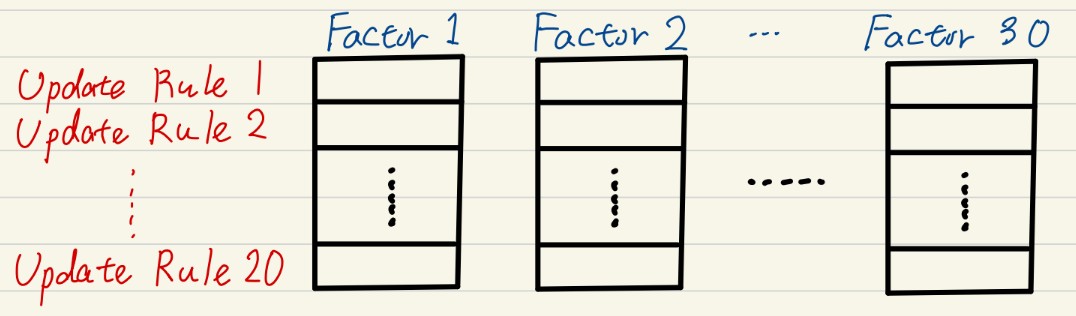
At the same time, because there are multiple variants of the sum–product algorithm, libraries such as ForneyLab and Infer.NET support several inference schemes, including Expectation Propagation, Variational Message Passing, and naive mean-field variational Bayes. This implies that each Factor subclass must implement multiple update rules, one for each inference algorithm.

Furthermore, if a library allows messages to be represented in different families—such as Gaussian, Gamma, Beta, categorical, or even particle-based messages—then the number of update rules per factor type increases even more.

(In my opinion, this is a fundamental limitation on the scalability of message passing libraries.)

What makes things even more complicated is that such a system must also include a mechanism that selects the correct update rule based on the graphical model specified by the user. You definitely do not want to write something like: “if … elif … elif … elif … elif … elif …”. In such situations, multiple dispatch in multimethod languages (such as Julia) is extremely helpful. A typical example is ForneyLab.jl. For instance, in ForneyLab/src/update_rules/addition.jl, all combination of the message types and applicable update rule for the addition factor (\(f(x,y,z) = \delta(z - (x + y))\)) are defined in a clean manner. In contrast, my project gPIE is focused on Gaussian messages to avoid this complexity.

3. Technical considerations and remaining challenges

This section highlights several technical challenges that arise when these algorithms are used in real-world applications.

Numerical issues

Algorithms such as Expectation Propagation are very powerful in many applications, but they lack general convergence guarantees, and are notoriously sensitive to numerical instability. A common heuristics to ensure convergence is to introduce damping-parameter and non-parallel scheduling, but choosing appropriate configuration before running EP is difficult. Adaptive-tuning of those parameters and schedules is an important aspect of message passing libraries.

Parallelism

Sum-product algorithm can benefit enormously from parallel computation. However, the scheduling—the order in which messages are updated—has an impact on the numerical stability of the iterative algorithm. A practical tension arises:

• Sequential (Gauss–Seidel–type) schedules often converge more robustly, but are inherently serial and slow.
• Parallel (Jacobi–type) schedules leverage modern hardware such as multi-core CPUs or GPUs, but tend to be far less stable for EP and loopy BP.

Finding schedules that strike a good balance—or adaptive schedules that switch strategies at runtime—is the current direction gPIE.

Interoperability with modern computational frameworks

Another practical issue is the relative isolation of message passing libraries from high-performance computational graph frameworks such as PyTorch, TensorFlow, and JAX. To mitigate this gap, gPIE adopts NumPy/CuPy as dual backends, enabling transparent switching between CPU and GPU execution.

References

Expectation Propagation for Approximate Bayesian Inference.
In UAI 2001, pp. 362–369.

Particle Methods as Message Passing.
In IEEE International Symposium on Information Theory (ISIT 2006), pp. 2052–2056.
https://doi.org/10.1109/ISIT.2006.261910

Variational Message Passing.
Journal of Machine Learning Research, 6, 661–694.

Pattern Recognition and Machine Learning.
Springer, New York.
ISBN: 978-0387310732.

Information, Physics, and Computation.
Oxford University Press.
https://doi.org/10.1093/acprof:oso/9780198570837.001.0001

Graphical Models, Exponential Families, and Variational Inference.
Foundations and Trends® in Machine Learning, 1(1–2), 1–305.
https://doi.org/10.1561/2200000001

A factor graph approach to automated design of Bayesian signal processing algorithms.
International Journal of Approximate Reasoning, 104, 185–204.
https://doi.org/10.1016/j.ijar.2018.11.002